
Deconvolution is a filtering process which removes a wavelet from the recorded seismic trace by reversing the process of convolution. The commonest way to perform deconvolution is to design a Wiener filter to transform one wavelet into another wavelet in a least-squares sense. By far the most important application is predictive deconvolution in which a repeating signal (e.g. primaries and multiples) is shaped to one which doesn't repeat (primaries only). Predictive deconvolution suppresses multiple reflections and optionally alters the spectrum of the input data to increase resolution. It is almost always applied at least once to marine seismic data.
The mathematical assumptions of predictive deconvolution are that:
While these assumptions are not satisfied by typical seismic data, extensive practical experience has shown that gapped predictive deconvolution can be very effective at suppressing multiple reflections with periods of less than around 300ms. The level of noise in the data can significantly affect deconvolution results. The following figure summarises deconvolution parameters and results using a simple synthetic example which consists of a water bottom reflection and series of multiple reflections. The objective of deconvolution would be to suppress the multiple reflections.
The mathematics of predictive deconvolution require that the autocorrelation of the source wavelet is known. Since this is rarely true in practice the autocorrelation of the seismic trace is used as an approximation instead. The autocorrelation function is critical in picking the deconvolution parameters of gap (also called minimum autocorrelation lag) and operator length (sometimes called maximum autocorrelation lag). Some contractors refer to the total operator length as the length of the gap plus the operator length, others refer (ambiguously) to this as the operator length.
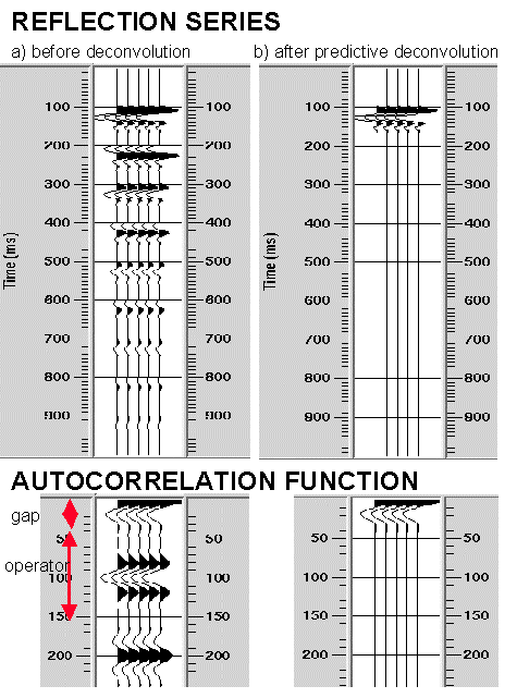
These parameters are summarised in the adjacent figure (a) and are usually defined in ms as multiples of the sample interval. Sometimes they are defined by the number of times that the autocorrelation crosses over the zero-line (zero-crossing). In the figure (a) the gap indicated would be the 3rd zero-crossing. The predictive deconvolution operator basically attempts to produce a trace with zero autocorrelation between the gap and operator length (b). There are no firm mathematical rules restricting the gap and operator length parameters, they are usually tested extensively and the processor and interpreter use their experience and judgement to pick the most pleasing section. As previously discussed a certain percentage of white noise is also required to stabilise the deconvolution calculations. For deconvolution to perform effectively the autocorrelation function of the trace used should be representative of the wavelet within the data. Extraneous noise and amplitude variations which may bias the autocorrelation should therefore be omitted from the computation. This is accomplished by choosing a design window for the autocorrelation function. Sometimes the wavelet varies sufficiently down the trace to require different deconvolution operators for the shallower and deeper parts of the section (multi-window deconvolution). An example from the North Sea would be to design one operator for the Tertiary section and one for the deeper Cretaceous/Jurassic section with the merge zone being selected above the Base Cretaceous reflector. This should be expected since we know higher frequencies are progressively removed from the wavelet as it travels though the earth by the processes of attenuation and absorption.
Gapped or Predictive Deconvolution is the commonest type of deconvolution. The method tries to estimate and then remove the predictable parts of a seismic trace (usually multiples). Predictive deconvolution can also be used to increase resolution by altering wavelet shape and amplitude spectrum. Spiking deconvolution is a special case where the gap is set to one sample and the resulting phase spectrum is zero.
Waveshaping deconvolution is designed to convert one wavelet into another. Examples include signature deconvolution where a mixed phase source signature is converted to it's minimum phase equivalent) and zero-phase conversion.
Since gapped predictive deconvolution requires a minimum phase input it is common to attempt to convert the data to minimum phase before further deconvolution is attempted. If the source wavelet were known or measured then this would be a trivial problem. In practise the source components are usually measured in the near field - that is very close to the airgun array. These measurements are sometimes included as auxiliary traces. What is required during processing is the signature recorded at the hydrophone - the so-called far-field signature. The far-field signature can be measured by a fixed hydrophone in deep water such as a facility in a Norwegian Fjord owned by PGS. The far-field signature can also be calculated from the near-field signature by a variety of methods mostly patented by GECO-PRAKLA. A number of software packages are available which can model the far-field signature from a given array of guns. In practice it has been shown (by contractors with vested interests) that modelled signatures compare favourably with those measured. Modelling is far cheaper than measurement. Therefore what is usually done is to obtain a modelled signature at the correct source depth and recorded sampling interval (this will be provided free by the acquisition contractor) and design an operator to convert this wavelet to minimum phase. This operator is then applied to the recorded seismic data prior to deconvolution. Note that this procedure does not take account of frequency losses as the wavelet travels through the earth. Modern seismic sources often consist of many airguns and since the input signature is approximately minimum phase the signature deconvolution stage rarely significantly changes the data. Nevertheless it should still be applied. For older source types such as vibroseis (land) or waterguns the signature deconvolution is an essential part of the data processing since the source is of mixed phase.
Note that a process used historically by GSI (then called HGS now called Western) called DESIG used to statistically extract a wavelet from each shot record and convert this to a zero-phase wavelet called "standard marine wavelet 6". They claimed to apply a zero-phase predictive deconvolution following this process so the resulting data would be approximately zero-phase (not minimum as standard). This type of process should be avoided since the results are unpredictable.
Predictive deconvolution applied prestack has historically been aimed at multiple suppression rather than wavelet compression. This is slightly strange since the multiple period is only fixed at zero-offset which is never recorded. In practice the deconvolution is applied trace by trace with a slightly different operator chosen for each trace. The method is referred to as DBS (deconvolution before stack). The amplitude relationships of the multiples should also be preserved prior to DBS by application of a geometrical spreading correction that does not use a primary velocity function. Theoretically the effects of attenuation (Q) should also be removed prior to deconvolution although the use of multi-windowed deconvolution should help to account for attenuation processes. It is important to remove as much noise as possible prior to deconvolution. The DBS often performs best after multiple suppression (e.g. RADON demultiple) and DMO which removes noise from the data. The order of DBS should therefore be tested. Transforming data to the tau-p domain will make the multiple period stationary, suppresses dipping noise and generally leads to improved DBS results.
In practise the DBS chosen is usually fairly conservative. This is because the job can largely be done by the DAS at a later stage in the processing where it is cheaper and easier to redo if the wrong parameters are chosen.
In many areas (e.g. the North Sea) a post-stack predictive deconvolution DAS (deconvolution after stack) is often applied in addition to that already applied prestack because the DBS does not attenuate multiples sufficiently well. Additionally the DAS can be used to perform any spectral enhancement which may have been undesirable prestack based on the premise that it is better to do these things later rather than earlier in the sequence. Post-stack the data should represent the near offset trace and the period of the multiple should be stable (ignoring alterations by the stacking process itself) and noise levels should be reduced. These features may enhance the effectiveness of deconvolution. The DAS is almost always applied before migration since the migration process itself may alter the period of the multiple reflections. However, sometimes the deconvolution is applied after migration (DAM). This would usually be because the DAS parameters could not be decided within the timeframe allowed. If the wrong parameters are chosen it is better to do it after an expensive process such as migration has already been applied. Sometimes the DAM is more effective because the migration reduces noise in the data. This route also may be preferred if target oriented multiple suppression routines such as SPLAT ä are to be applied. On some data, particularly in deep water where heavy multiple suppression routes have been attempted, the use of DAS may not be required and should be replaced by spectral whitening methods.
Unfortunately there are few easy guidelines here.
The appropriate DAS parameters should be selected by trials usually established by the contractor. Previous experience in the data area is also useful since usually the trials are designed around some initial guess at the final parameters. A section, or more usually a portion of section of 500 traces, would be taken and run through a series of trials displayed side by side at fixed gain level. If a bandpass filter or AGC is applied following the trials then an ungained or raw version should also be displayed for reference. The autocorrelation functions associated with the deconvolution parameters should also be displayed. The following figures show examples of DAS trials. The processor and interpreter would use their skill and judgement to pick the optimum parameters for the data. It is also sensible to note that if the data is required to tie other vintages then it is wise to check the parameters applied to these vintages since a mis-match could result in change of character of a target event which could conceivably lead to mis-interpretation.
The deconvolution gap probably has the most effect on the final appearance of the deconvolved data. It must be remembered that the choice of gap will effect the resulting amplitude spectrum of the data. A shorter gap will cause more wavelet compression or spectral whitening and will boost any high and lower frequency noise present. The spike deconvolution affords maximum resolution, is often too noisy, but should always be tested, even if only as a reference section. Some schools of thought prefer to choose a different DAS gap to that used for the DBS to avoid too much spectral alteration of the same frequency bands.
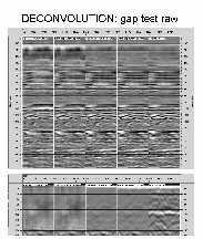
The adjacent figure compares (left to right) gaps of 4ms (spike), 12ms, 16ms, 24ms and raw. Click here to enlarge the figure. The upper display shows the deconvolved results and the lower display shows the associated enlarged autocorrelation functions. When using PROMAX (as in many processing systems) two jobs must be run and the displays merged. Some contractors may be lazy on this, but it is essential to display the autocorrelation functions. The autocorrelation of the wavelet is seen to be around 20ms on panel 5. The spike deconvolution and the 12ms gap are seen to undesirably boost low frequency noise in the shallower part of the section. The 16ms and 24ms gap produce very similar results. The 16ms gap would probably be the optimum compromise between spectral enhancement and boosting noise. For deeper targets a 24ms or 32ms gap is probably the commonest used in the North Sea. After stack the high frequency noise has generally been reduced so if the data are whitened too much then generally it is the lower frequencies which are observed (panels 1 & 2). In this case it may be more desirable to apply a bandpass filter following deconvolution.
Deconvolution operator length will have the most effect on the degree of multiple suppression performed by the predictive deconvolution. Assuming that the dominant multiple period is the seabed multiple then operator lengths less than the water bottom (e.g. 100ms) will generally just perform spectral whitening/wavelet compression. Longer operator lengths (e.g. water bottom + 60ms) will generally be effective at multiple suppression. Operators longer than this may start to deconvolve geology. Deconvolution will generally have a poor performance on multiples with periods greater than 300ms.
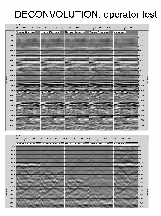
The adjacent figure uses a 16ms gap and from left to right the following operator lengths 80ms, 120ms, 160ms, 240ms and no DAS. Click here to display an enlarged figure. The upper display shows the deconvolved data and the lower panel the associated autocorrelation functions. Both panels have been reduced slightly in size in order to create the figure. The autocorrelation from panel 5 shows that the dominant multiple period is around 110ms. Panel 1 provides just wavelet compression and no multiple suppression. Panels 2 and 3 are very similar in results for multiple suppression. It is noted that the residual multiple is not particularly strong on this data example.
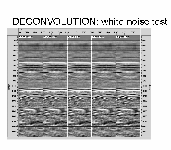
The adjacent figure shows the effects of varying white noise percentage on the chosen deconvolution parameters of 16ms gap, 160ms operator. Click here for an enlarged display. Parameters tested are (left to right) 0.1%, 0.5%, 2%, 5% and no DAS. As shown in these displays (and generally found) the white noise percentage does not significantly alter the effectiveness of the deconvolution. 0.1% to 1% is the commonest used. For noisy data an increased percentage of white noise can be used to improve the deconvolution results.
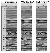
As noted above, the application of a bandpass filter following deconvolution may sometimes help to reduce the low and high frequency noise boosted by short gap deconvolution whilst maintaining the extra resolution obtained from the signal. The adjacent figure (click here for an enlargement) shows the filtered spiking deconvolution, the raw 16ms gap and the filtered 16ms gap deconvolution. The filtering is seen to reduce the low frequency noise in the upper part of the section and the resolution afforded by the spike is seen, in this case not to be superior to that of the filtered 16ms gap (c). Indeed while the latter deconvolution has better signal content in the deeper section the spike deconvolution (a) generally is richer in lower frequencies. The optimum deconvolution and filter choices are, as ever, a matter of personal preference and will ultimately be decided by the interpreter and processor in conjunction. Note that there is a phase difference between the spike (which is zero-phase) and the gap (minimum phase) deconvolution results. There are some schools of thought which state that the migration will perform better if the input data has had spike deconvolution applied but there is little theoretical background for this. Generally in the North Sea data is too noisy for spike deconvolution to be effective even when followed by bandpass filtering.
Occasionally a deconvolution operator and gap may be designed to attenuate a particular multiple period within the data only. This technique might be used for very deep water. Typically a long gap e.g. water bottom -60ms would be used with an operator length of water bottom + 60ms. The results of this procedure can be quite unpredictable and should be avoided if possible. This method is commonly used as a DBS in the processing of site survey data when preceded by an NMO correction at water velocity in order to stabilise the multiple period.